
Highlight
MLX Swift brings NumPy-style n-dimensional array operations and automatic differentiation natively to Swift, so numerical computing code can be written in a mathematical style and executed in parallel on the GPU.
Core Content
The pain of numerical computing in Swift
Developers doing scientific computing or machine learning on Apple platforms have long faced an awkward choice: write low-level vector operations with Accelerate, hand-write GPU kernels with Metal Performance Shaders, or switch to the Python ecosystem. Swift itself lacked a high-level, expressive numerical computing tool. Matrix multiplication is manageable, but once you need physical simulation, iterative solvers, or model training, the code fills with boilerplate unrelated to the math.
MLX Swift changes this. Its core design is inspired by NumPy: the central abstraction is an n-dimensional array (MLXArray), and operations apply to whole arrays rather than individual scalars. If you have used NumPy, moving to MLX Swift has almost no learning curve.
Lazy evaluation: wait until the last moment
One key MLX Swift feature is lazy evaluation. Every addition, subtraction, multiplication, or division you apply to an array is not executed immediately. Instead, it builds a compute graph. Only when you call eval() or read a concrete value is the whole graph submitted to the GPU.
The benefit is operator fusion. Launching GPU kernels has overhead, so fusing many small operations into one larger kernel can significantly improve performance on Apple Silicon. The cost is that developers must manage when to call eval(), especially inside loops. Otherwise, the compute graph can grow without bound and exhaust memory.
Automatic differentiation: from loss to gradient in one line
The heart of model training is gradient descent, and gradient descent requires gradients. In the past, implementing this in Swift meant either deriving gradients by hand or relying on compiler-level efforts such as Swift for TensorFlow. MLX Swift solves it with the function transform grad(): pass in a forward loss function, and it returns a function that automatically computes gradients. MLX performs the derivation underneath, without requiring you to write derivative code.
Details
Matrix operations and power iteration (03:04)
The session opens with the classic power iteration algorithm to demonstrate basic MLX Swift usage. The goal is to find the largest eigenvalue of a symmetric matrix and its corresponding eigenvector.
import MLX
let n = 100
let steps = 10
let B = MLXRandom.normal([n, n])
var v = MLXRandom.normal([n])

// Construct the symmetric matrix A = B^T + B
let A = B.T + B

// Power iteration: v <- A v / ||A v||
for _ in 0 ..< steps {
    let Av = matmul(A, v)
    v = Av / norm(Av)
    eval(v)  // Force evaluation at each step to prevent graph growth
}

// Recover the eigenvalue: lambda = v^T A v
let lambda = matmul(matmul(v.T, A), v)
print(lambda)
Key points:
B.Ttakes the transpose, and+performs matrix addition. The code maps directly to the mathematical formula.matmulperforms matrix multiplication, andnormcomputes the L2 norm.eval(v)must be called inside the loop; otherwise each iteration keeps appending nodes to the compute graph.- Reading
lambdaat the end triggers lazy evaluation and automatically completes all pending operations.
Mandelbrot fractal: from scalar loops to array operations (05:09)
The Mandelbrot set is a classic example for showing the power of array computing. For each point c on the complex plane, iterate z = z^2 + c. If the magnitude never exceeds 2, the point belongs to the set.
A pure Swift scalar implementation needs nested loops and computes one pixel at a time:
// Pure Swift, scalar-by-scalar computation
var counts = Array2D<Int>(width: w, height: h)

for y in 0 ..< h {
    for x in 0 ..< w {
        let c = Complex(xMin + Float(x) * xStep, yMin + Float(y) * yStep)
        var z = Complex<Float>.zero
        var limit = maxIterations
        for i in 0 ..< maxIterations {
            z = z * z + c
            if z.lengthSquared > radiusSquared {
                limit = i
                break
            }
        }
        counts[x, y] = limit
    }
}
The MLX Swift version treats the entire grid as one array:
import MLX

let x = linspace(-2.0, 0.5, count: w)
let y = linspace(-1.25, 1.25, count: h).reshaped(h, 1)
let c = x + y.asImaginary()

var z = MLXArray.zeros(like: c)
var counts = MLXArray.zeros(c.shape, dtype: .int16)

for _ in 0 ..< maxIterations {
    z = z * z + c                       // Iterate over the entire grid at once
    counts = counts + (abs(z) .< 2)     // Count iterations that have not escaped
}
Key points:
linspacecreates evenly spaced sequences, andreshapedadjusts dimensions for broadcasting.y.asImaginary()converts a real-valued array into the imaginary component, then adds it toxto form a complex grid.z = z * z + capplies to the whole array at once, with no manual per-pixel traversal.abs(z) .< 2produces a Boolean mask and counts how many iterations each point remains within the boundary.- GPU execution is used by default and can be more than 10x faster than a scalar CPU implementation.
Heat diffusion simulation: convolution and boundary conditions (07:27)
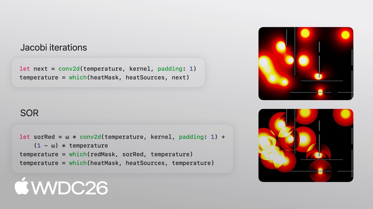
Heat diffusion demonstrates how to handle scenarios where each cell interacts with its neighbors. The core idea of Jacobi iteration is that each cell’s new temperature equals the average of its four neighbors.
// Convolution kernel: 0.25 in each of the four directions, 0 at the center
let kernel = MLXArray(converting: [
    0,    0.25, 0,
    0.25, 0,    0.25,
    0,    0.25, 0,
]).reshaped(1, 3, 3, 1)

var temperature = heatSources

// Loop until convergence
let next = conv2d(temperature, kernel, padding: 1)
temperature = which(heatMask, heatSources, next)
Key points:
conv2dapplies the convolution kernel to the whole grid at once, replacing hand-written neighbor traversal.whichis an element-wise ternary operator: ifheatMaskis true (heat source or wall), keep the fixed value; otherwise use the convolution result.padding: 1keeps the output size the same as the input after convolution.
Jacobi iteration is fast per step but converges slowly, because heat can move only one cell per iteration. The session then introduces Successive Over-Relaxation (SOR), which speeds convergence with an over-relaxation parameter omega:
let omega: Float = 2.0 / (1.0 + sin(Float.pi / Float(max(M, N))))

let redMask   = checkerboard(rows: M, cols: N, phase: 0)
let blackMask = checkerboard(rows: M, cols: N, phase: 1)

// Update red cells using the old values of black neighbors
let sorRed = omega * conv2d(temperature, kernel, padding: 1) + (1 - omega) * temperature
temperature = which(redMask, sorRed, temperature)
temperature = which(heatMask, heatSources, temperature)

// Update black cells using the new values of red neighbors
let sorBlack = omega * conv2d(temperature, kernel, padding: 1) + (1 - omega) * temperature
temperature = which(blackMask, sorBlack, temperature)
temperature = which(heatMask, heatSources, temperature)
Key points:
omegais computed from the grid size and can reduce convergence iterations from O(N^2) to O(N).- Red-black checkerboard masks implement an “almost in-place update”: red cells update while black neighbors still hold old values, and black cells update after red neighbors have refreshed.
- In the session demo, SOR is much faster than Jacobi, so much so that the animation had to be slowed down 100x to make the process visible.
Curve fitting and automatic differentiation (11:13)
The final example shows MLX Swift’s automatic differentiation. Given a set of data points, fit a quadratic polynomial. The core code looks like this:
// Define the prediction function
func f(_ theta: MLXArray) -> MLXArray {
    theta[0] + theta[1] * x + theta[2] * x ** 2
}

// Define the mean-squared-error loss
func loss(_ theta: MLXArray) -> MLXArray {
    mean((f(theta) - y) ** 2)
}

var theta = zeros([numParams])
let gradLoss = grad(loss)  // Automatically get the gradient function

for _ in 0 ..< steps {
    let g = gradLoss(theta)          // Gradient of L(theta)
    theta = theta - learningRate * g // Parameter update
    eval(theta)                      // Force evaluation and truncate the graph
}
Key points:
grad(loss)converts the loss function into a function that returns gradients, with no hand-written derivatives.gradLoss(theta)automatically computes each parameter’s partial derivative of the loss through backpropagation.eval(theta)at the end of the loop both performs computation and frees memory. Omitting it can cause OOM.- This mechanism is the foundation for training all machine-learning models, and MLX Swift reduces it to a few lines of code.
MLX’s complete toolbox (12:17)
The session closes by listing MLX’s full capability matrix: linear algebra, FFT, n-dimensional convolution, reductions, scan and prefix sums, indexing and slicing, random number generation, and more. These operations share the same lazy evaluation and automatic differentiation infrastructure.
Core Takeaways
-
On-device physics simulation apps: Use
conv2dpluswhichto implement fluid, heat, or electric-field simulations. MLX Swift’s GPU acceleration makes real-time rendering of complex physical effects possible on phones. Entry APIs:MLXArray,conv2d,which. -
Custom image-filter pipelines: Use array-level operations and FFT to implement CNN-style image processing, such as style transfer or super-resolution. MLX Swift’s lazy evaluation automatically fuses multiple filter operations into a small number of GPU kernels. Entry APIs:
MLXArray.fft,conv2d. -
On-device model fine-tuning tools: Based on
mlx-swift-lmandgrad(), fine-tune language models on device with small sample datasets. MLX Swift’s automatic differentiation lets the training loop be written directly in Swift without cross-language calls. Entry APIs:grad(), themlx-swift-lmrepository. -
Real-time audio signal processing: Use FFT and array operations for spectrum analysis, filter banks, or audio effects. MLX Swift’s GPU parallelism can process multiple audio streams at the same time. Entry APIs:
MLXArray.fft, element-wise operations. -
Interactive math visualization: Extend the Mandelbrot set to Julia sets, Newton fractals, and more. Build the interface in SwiftUI and use MLX Swift for background computation. GPU acceleration supports real-time zooming and panning. Entry APIs:
linspace,reshaped, complex-number operations.
Related Sessions
- Session 232: Bring local AI to your apps with MLX - An introduction to using MLX for on-device AI inference
- Session 233: Scale MLX to multiple devices - Distributed MLX training across multiple devices
- Session 330: Accelerate machine learning with Metal tensors - Tensor acceleration primitives at the Metal layer
- Session 262: What’s new in Swift - New Swift language features and how they work with MLX Swift’s type system
- Session 279: What’s new in RealityKit - Real-time physics simulations in 3D scenes can be combined with MLX
Comments
GitHub Issues · utterances