
Highlight
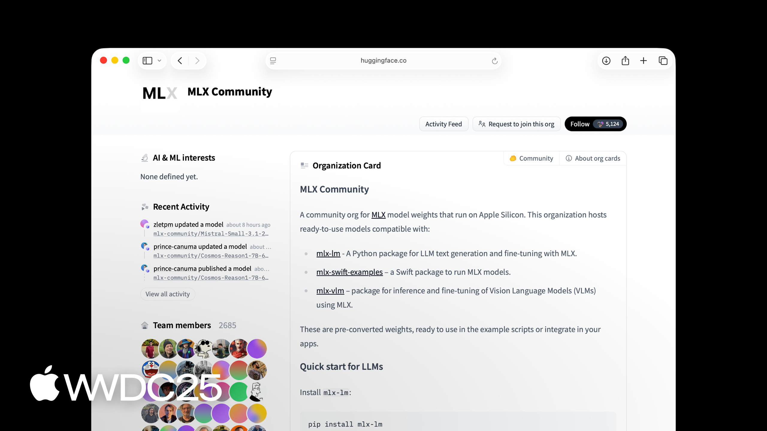
MLX is an open-source array framework built by Apple, designed for the unified memory architecture of Apple Silicon. The core idea is radical: CPU and GPU share memory; no manual data copying is needed.
Core Content
If you have ever run PyTorch on a Mac, you have probably been annoyed by one thing: the CPU and GPU sit on the same chip, yet model tensors still have to shuttle back and forth between two “virtual” memory pools. Every .to("mps") is a copy, and large-model inference often runs out of GPU memory. MLX, introduced by Apple at WWDC 2025, was built to fix this.
MLX flips the old rule of “compute chases data.” In traditional frameworks, an array in CPU memory can only be computed on the CPU, and an array in GPU memory can only be computed on the GPU. MLX places arrays in the unified memory of Apple Silicon, so they no longer belong to a specific device. Instead, each op specifies where it runs via stream=mx.cpu or stream=mx.gpu. The same data can be operated on by CPU and GPU in parallel, and the framework manages dependencies automatically. On top of this foundation, MLX bundles NumPy-style APIs, PyTorch-style nn.Module, and JAX-style function transforms (mx.grad, mx.compile) into a single package, letting you run the same code on Mac, iPhone, iPad, and Vision Pro, with Python, Swift, C++, and C APIs all covered.
Detailed Content
Installation and Basic Array Operations (03:48). After a one-line pip3 install mlx, the API is almost identical to NumPy:
import mlx.core as mx

# Make an array
a = mx.array([1, 2, 3])

# Make another array
b = mx.array([4, 5, 6])

# Do an operation
c = a + b

# Access information about the array
shape = c.shape
dtype = c.dtype

print(f"Result c: {c}")
print(f"Shape: {shape}")
print(f"Data type: {dtype}")
Key points:
import mlx.core as mx: the core array library of MLX; naming conventions follow NumPy.mx.array([...]): creates an array from a Python list; data lives in unified memory, with no device concept.a + b: operator overloading; the returnedcis a lazy, unevaluated array (see below).c.shape,c.dtype: same names and meanings as NumPy; existing NumPy knowledge transfers directly.
Unified Memory Programming (05:31). This is the biggest difference between MLX and other frameworks: the stream parameter lives on the op, not on the array:
import mlx.core as mx

a = mx.array([1, 2, 3])
b = mx.array([4, 5, 6])

c = mx.add(a, b, stream=mx.gpu)
d = mx.multiply(a, b, stream=mx.cpu)

print(f"c computed on the GPU: {c}")
print(f"d computed on the CPU: {d}")
Key points:
aandbare the same data; there is no “on CPU or GPU” question.mx.add(a, b, stream=mx.gpu): runs the addition on the GPU.mx.multiply(a, b, stream=mx.cpu): the same input, but the multiplication runs on the CPU.- The two ops have no dependency, so they can run in parallel; if there is a dependency, MLX orders them automatically.
Lazy Evaluation (06:20). When MLX calls an op, it only builds the computation graph; it does not actually run anything:
import mlx.core as mx

a = mx.array([1, 2, 3])
b = mx.array([4, 5, 6])
c = a + b

# Evaluates c before printing it
print(c)

# Also evaluates c
c_list = c.tolist()

# Also evaluates c
mx.eval(c)
Key points:
c = a + bdoes not trigger computation; it only adds an addition node to the graph.print(c),.tolist(), ormx.eval(c)each force evaluation; if the result is never used, the computation is skipped entirely.- This leaves room for graph optimization, such as fusing multiple ops into a single kernel.
Function Transforms: Automatic Differentiation (07:32). mx.grad turns a function into a new function:
import mlx.core as mx

def sin(x):
    return mx.sin(x)

dfdx = mx.grad(sin)

d2fdx2 = mx.grad(mx.grad(mx.sin))

# Computes the second derivative of sine at 1.0
d2fdx2(mx.array(1.0))
Key points:
mx.grad(sin)returns the differentiated functiondfdx, which is itself still a function.- Function transforms nest arbitrarily:
mx.grad(mx.grad(...))gives the second derivative directly. - This style comes from JAX, and it works well for training models and computing gradients.
Building Neural Networks with mlx.nn (09:16):
import mlx.core as mx
import mlx.nn as nn
import mlx.optimizers as optim

class MLP(nn.Module):
    """A simple MLP."""

    def __init__(self, dim, h_dim):
        super().__init__()
        self.linear1 = nn.Linear(dim, h_dim)
        self.linear2 = nn.Linear(h_dim, dim)

    def __call__(self, x):
        x = self.linear1(x)
        x = nn.relu(x)
        x = self.linear2(x)
        return x
Key points:
nn.Moduleis the base class for all layers and containers; it provides parameter access, loading, saving, and other methods.- Standard layers such as
nn.Linearandnn.reluhave names and signatures that match PyTorch conventions. - Note that MLX uses
__call__instead of PyTorch’sforward— this is one of only two differences from PyTorch.
Fusing Kernels with mx.compile (11:35). Add the decorator, and multiple element-wise ops get fused into a single GPU kernel, cutting redundant memory round-trips and kernel launch overhead:
import mlx.core as mx
import math

def gelu(x):
    return x * (1 + mx.erf(x / math.sqrt(2))) / 2

@mx.compile
def compiled_gelu(x):
    return x * (1 + mx.erf(x / math.sqrt(2))) / 2
Key points:
gelucontains four ops (erf, division, addition, multiplication), which originally map to four separate kernel launches.@mx.compilelets MLX compile these nodes into a single kernel.- The payoff is biggest for small functions called repeatedly, such as activation functions and normalization.
mx.fast High-Performance Ops (12:32). Several core Transformer ops (RMS Norm, SDPA, RoPE) have hand-optimized versions; using them directly is much faster than building them yourself. Custom Metal Kernels (13:30) let you embed Metal shader source directly into the computation graph:
import mlx.core as mx

source = """
    uint elem = thread_position_in_grid.x;
    out[elem] = metal::exp(inp[elem]);
"""
kernel = mx.fast.metal_kernel(
    name="myexp",
    input_names=["inp"],
    output_names=["out"],
    source=source,
)

x = mx.array([1.0, 2.0, 3.0])
out = kernel(
    inputs=[x],
    grid=(x.size, 1, 1),
    threadgroup=(256, 1, 1),
    output_shapes=[x.shape],
    output_dtypes=[x.dtype],
)[0]
Key points:
sourceis raw Metal code;thread_position_in_gridis a standard Metal built-in variable.mx.fast.metal_kernel(...)wraps this source into a callable object.- At call time,
gridandthreadgroupspecify thread layout, andoutput_shapes/output_dtypesdescribe the output tensor. - Use this to hand-write extreme optimizations for ops not covered by MLX, while still enjoying lazy graph scheduling.
4-bit Quantization (14:41). mx.quantize packs weights into 4-bit, and mx.quantized_matmul handles inference; at the model level, nn.quantize(model, bits=4, group_size=32) replaces all Linear/Embedding layers in one line. Multi-Machine Distributed Training (16:50) uses mx.distributed.init() to get a group, then collective communication primitives such as mx.distributed.all_sum, together with mlx.launch --hosts ip1,ip2,ip3,ip4 my_script.py to run the same code across multiple Macs linked by Ethernet or Thunderbolt.
MLX Swift (18:20). The same API is translated into Swift, making it easy to integrate into iOS and macOS apps:
import MLX

let a = MLXArray([1, 2, 3])
let b = MLXArray([1, 2, 3])
let c = a + b

let shape = c.shape
let dtype = c.dtype
Key points:
MLXArraycorresponds to Python’smx.array; construction is the same.- Operator overloading and attribute names (
shape,dtype) stay consistent, making cross-language migration easy. - It can be bundled directly on iOS, iPadOS, and visionOS, with no extra runtime dependency.
Core Takeaways
-
What to do: Move existing PyTorch inference on Mac to MLX, and measure the latency gains from unified memory.
- Why it matters: the MPS backend’s copy and sync overhead is significant on large models; MLX skips the “move data” step, and 4-bit quantization is built in.
- How to start: pick a 7B-scale model, find the matching weights in the MLX LM repo; quantize with
nn.quantize(model, bits=4, group_size=32), then compare tokens/s and peak memory.
-
What to do: Wrap activation functions and normalization in your training loop with
@mx.compile.- Why it matters: these functions are called repeatedly, and each call goes through multiple kernels; after fusion, you save launch overhead, which is the easiest speedup to capture.
- How to start: first replace hand-written versions with
mx.fast.rms_norm,mx.fast.scaled_dot_product_attention, and other ready-made implementations; for any remaining small functions, add the@mx.compiledecorator.
-
What to do: Chain two or three Mac minis into a local distributed cluster over Thunderbolt.
- Why it matters: compared to stuffing a single machine with GPU memory, horizontal scaling lets you run larger models, and MLX’s
mlx.launchcompresses startup complexity into a single command. - How to start: install MLX on each machine, use
mx.distributed.init()to get a group, write a minimalall_sumdemo to verify connectivity; then plug your existing training script intomlx.launch --hosts.
- Why it matters: compared to stuffing a single machine with GPU memory, horizontal scaling lets you run larger models, and MLX’s
-
What to do: Embed MLX Swift into an iOS or visionOS app for on-device inference.
- Why it matters: unlike Foundation Models, MLX lets you bring your own model weights and graph structure, which is the most friendly option for self-trained or community models.
- How to start: clone a minimal inference example from the
mlx-swift-examplesrepo, swap the model weights for your own Hugging Face MLX community version, get it running, then wire it into SwiftUI.
Related Sessions
- Bring advanced speech-to-text to your app with SpeechAnalyzer — overall design and integration of the SpeechAnalyzer on-device speech recognition API.
- Code-along: Bring on-device AI to your app using the Foundation Models framework — adding generative AI features to a SwiftUI app with the Foundation Models framework.
- Deep dive into the Foundation Models framework — guided generation, tool calling, and other advanced uses of Foundation Models.
- Design interactive snippets — interactive snippet design patterns for App Intents.
Comments
GitHub Issues · utterances